PreprintUnder double-blind reviewOAIZIB-CM · n=102
MBEDNet
A Mamba–CNN network with dual edge-guided decoders for segmentation of tibiofemoral bone and cartilage.
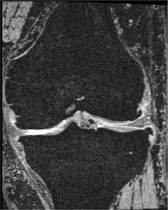
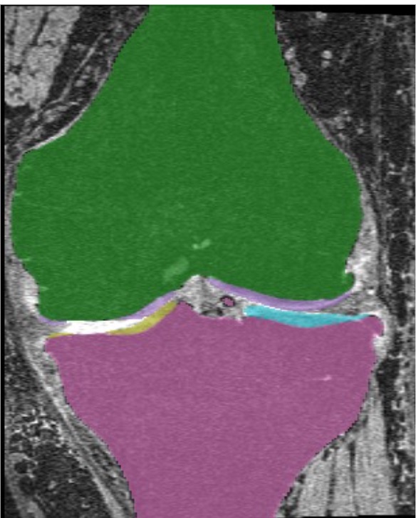
Sagittal · 0.365 × 0.365 × 0.7 mm
Scroll
A Mamba–CNN network with dual edge-guided decoders for segmentation of tibiofemoral bone and cartilage.
Volumetric knee MRI at 0.365 × 0.365 × 0.7 mm. The articular cartilage running between femur and tibia is two to three voxels thick and barely separable from the bone beneath it.
MBEDNet labels femoral and tibial bone plus femoral, medial and lateral tibial cartilage — a semantic decoder and a boundary decoder running together, so the bone–cartilage interface is predicted rather than inferred from region overlap.
The predicted mask converts to triangular meshes. Eight femoral landmarks localised on those meshes land within 0.964 mm of the ground truth — the geometry a patient-specific implant is planned against.
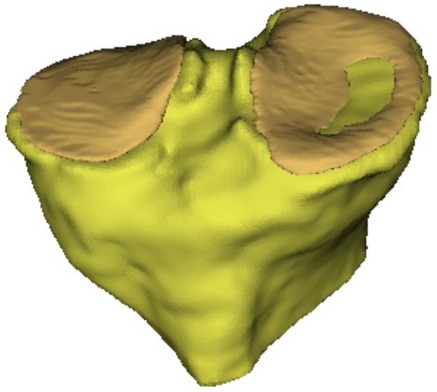
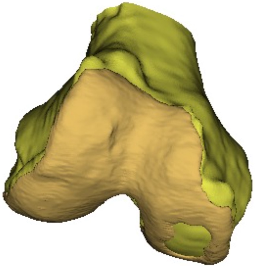
Preoperative 3D segmentation of the tibiofemoral joint guides image-based Total Knee Arthroplasty (TKA) and supports the design of patient-specific implants. Automated 3D segmentation in TKA still remains challenging due to thin, low contrast cartilage layers between the tibiofemoral bone structures.
We propose Mamba Edge-Net (MBEDNet), which integrates the local feature extraction of convolution with long dependency modelling of Mamba to effectively and efficiently segment tibiofemoral anatomies, with sharp contrast between bone and cartilage. MBEDNet is lightweight while achieving the highest average Dice similarity coefficient among compared state-of-the-art architectures, several of which require 1.3 to 5.5 times more parameters. The network is also optimized to handle severe osteophytes of Kellgren–Lawrence grade IV.
Evaluated on the publicly available OAIZIB-CM knee MRI dataset, MBEDNet reaches Dice scores of 98.46% and 98.64% on the femur and tibia, and 89.03% and 86.29% on femoral and tibial cartilage.
Accurate TKA relies on precise segmentation of the femur, tibia and the articular cartilage around them — and manually tracing those joint lines across slices is laborious. Automating it runs into a split requirement: the cartilage–bone interface needs voxel-level acuity, while femur–tibia alignment needs the whole volume in view. No single backbone family gives both.
| Backbone family | Receptive field | Complexity | Weak point |
|---|---|---|---|
| Convolutional U-Nets | Local | Linear | Cannot model femur–tibia spatial relations |
| Vision Transformers | Global | O(N²) in tokens | Prohibitive on volumes; weak fine detail |
| Swin / windowed attention | Windowed | Reduced | Buys efficiency by giving up long-range context |
| State space models (Mamba) | Global | Linear | State averaging smooths out voxel-level structure |
MBEDNet’s answer is not to pick one. Each encoder stage runs a convolutional branch and a state-space branch in parallel and fuses them, and a second decoder is dedicated entirely to boundaries — so the interface evidence the state-space path smooths away is reconstructed by a stream built to find it.
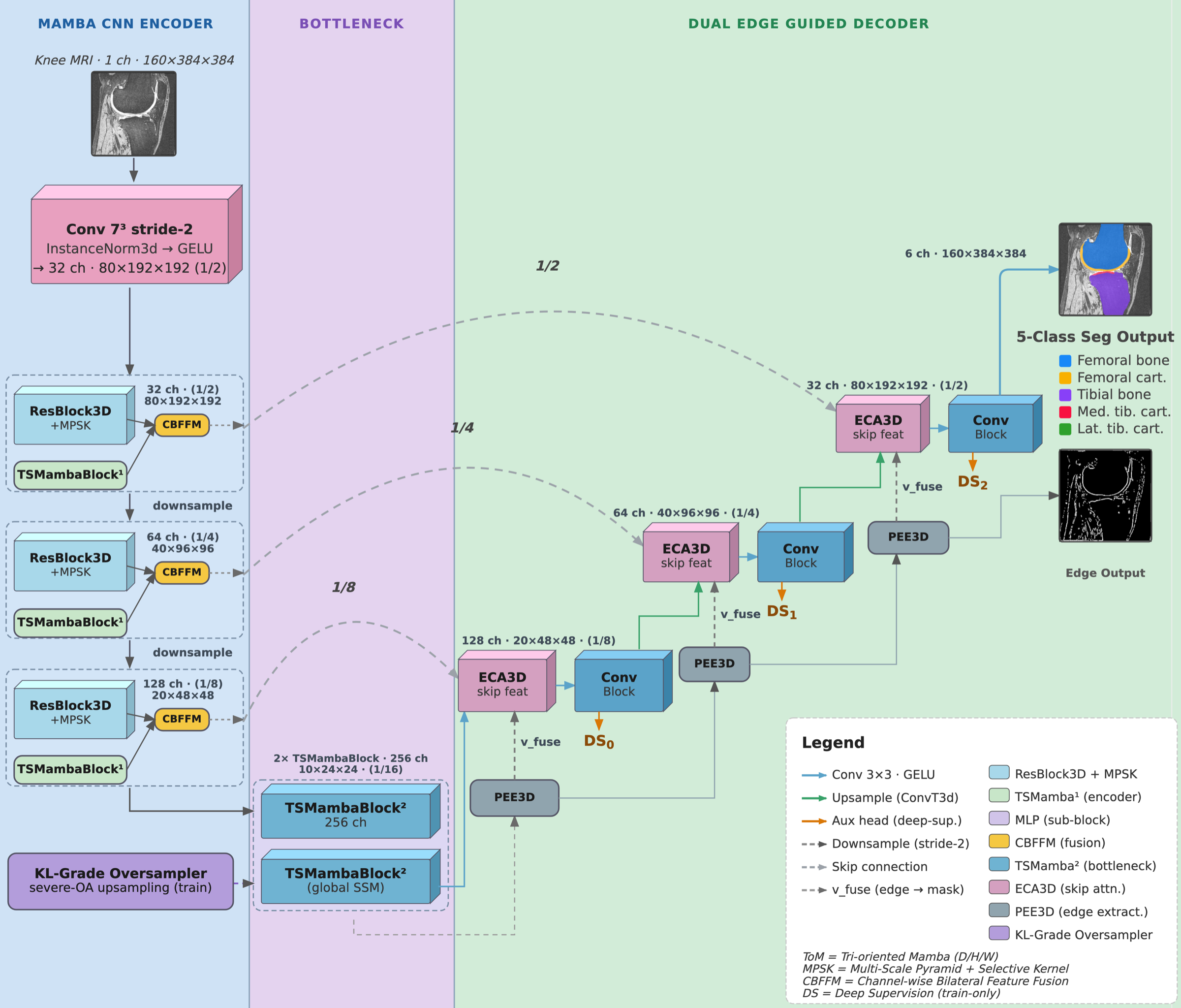
A 7×7×7 convolution lifts the volume to 32 channels and halves every spatial dimension, giving (32, D/2, H/2, W/2) before the first encoder stage.
The volume is refined three times, once along each axis. Each pass keeps selective state deciding what to retain or discard; the three scans merge through a 1×1×1 convolution and instance norm.
Three separate passes keep the cost linear at O(D + H + W) each — against O((D × H × W)²) for full 3D self-attention.
Parallel 3D convolutions at 1³, 3³ and 5³ feed a learned per-channel selective-kernel mechanism, so the network uses small kernels for thin cartilage texture and large ones for bone. Pyramid pooling at 2×2, 4×4 and 8×8 adds multi-scale context.
The branches concatenate, pass through a 1×1×1 convolution, GELU and instance norm to give Z, then gate by a squeeze-and-excitation weight. The result serves both as the encoder skip and as the next stage’s input, after a stride-2 downsample doubling the channels (32 → 64 → 128).
Two stacked TSMambaBlocks model relative femur–tibia alignment. Fine boundary detail is reintroduced downstream by the skips and the edge decoder.
At each of three upscaling stages, a stride-2 transposed convolution concatenates with an ECA-recalibrated skip and is refined by two 3×3×3 conv → GELU → IN blocks.
The boundary stream takes the raw, un-gated skip — ECA’s recalibration would attenuate exactly the high-frequency content the extractor needs. A Progressive Edge Extractor subtracts multi-scale low-pass responses (3D average pooling, k ∈ {3, 5}) from a squeezed feature to expose scale-specific unsharp detail.
Boundary evidence is injected into the semantic stream in one direction only, at every decoder level, and the fused representation is what propagates onward. That matters most for cartilage spanning two to three voxels, where region overlap alone is ambiguous.
MBEDNet matches the larger MSPF-VM-Unet with 23% fewer parameters, and its cartilage-focused training improves cartilage segmentation by roughly 1–2% over SwinUNETR. Boundary-aware Mamba encoders capture thin-structure geometry more effectively than pure transformer or heavier Mamba–CNN architectures.
MBEDNet in blue, baselines in grey. Up and to the left is better.
| Method | Params | FB | TB | FC | TC | Avg |
|---|---|---|---|---|---|---|
| U-Net | 31.0 M | 96.43 | 96.05 | 84.73 | 83.21 | 90.11 |
| V-Net | 71.0 M | 97.04 | 96.52 | 87.75 | 84.09 | 91.35 |
| nnU-Net | 30.0 M | 97.87 | 97.17 | 88.51 | 85.49 | 92.26 |
| I-Mask-RCNN | 44.0 M | 97.60 | 97.53 | 83.32 | 80.67 | 89.78 |
| SwinUNETR | 62.2 M | 98.46 | 98.47 | 87.77 | 84.47 | 92.29 |
| MtRA-Unet | 96.5 M | 98.53 | 98.44 | 89.19 | 86.02 | 93.05 |
| VM-UNet | 27.0 M | 97.35 | 96.31 | 85.33 | 83.17 | 90.54 |
| MSPF-VM-Unet | 22.7 M | 98.61 | 98.37 | 89.57 | 85.63 | 93.05 |
| MBEDNet (ours) | 17.4 M | 98.46 | 98.64 | 89.03 | 86.29 | 93.11 |
Read this carefully. Baseline results are 5-fold cross-validation means reproduced from the MSPF-VM-Unet paper; MBEDNet and SwinUNETR were each trained on OAIZIB-CM under the same protocol with separate independent splits, and MBEDNet is evaluated on our held-out test set (n=102). No significance testing is reported for this table — without per-case predictions under a matched protocol, the paired, fold-dependence-aware inference a valid comparison requires is not possible. FB femoral bone · TB tibial bone · FC femoral cartilage · TC tibial cartilage, the mean of medial and lateral.
Removing the Mamba branch costs the most, confirming that global context is essential for joint segmentation; removing the edge decoder degrades HD95 specifically, reflecting its role in preserving thin cartilage boundaries.
Change in five-class mean DSC against the full model (92.00%). Percentage points.
| Configuration | DSC ↑ (%) | HD95 ↓ (mm) | ASSD ↓ (mm) |
|---|---|---|---|
| w/o Mamba branch | 89.80 | 1.44 | 0.400 |
| w/o Edge decoder | 90.70 | 1.29 | 0.360 |
| w/o Bottleneck (Mamba → conv) | 91.00 | 1.14 | 0.330 |
| w/o Edge loss | 91.60 | 1.03 | 0.310 |
| Full model | 92.00 | 0.95 | 0.289 |
HD95 — 95th percentile Hausdorff distance. ASSD — average symmetric surface distance. Table 2 averages over all five annotated classes, so its DSC is not directly comparable with the four-structure average in Table 1. Model differences were assessed on per-case Dice with a two-sided Wilcoxon signed-rank test paired across the 102 held-out cases; per-structure p-values were Holm–Bonferroni corrected.
Scores hold up across KL grades, with a modest decline at grade IV where cartilage degradation is most pronounced and small spurious voxels occasionally appear near severely eroded interfaces.
Higher is better. Sample sizes below each grade.
Lower is better. Millimetres.
| KL grade | n | FB | TB | FC | TC | Avg DSC | HD95 | ASSD |
|---|---|---|---|---|---|---|---|---|
| 0 | 20 | 98.76 | 98.82 | 88.62 | 85.99 | 93.05 | 0.73 | 0.149 |
| 1 | 12 | 98.74 | 98.71 | 89.74 | 88.06 | 93.81 | 0.70 | 0.141 |
| 2 | 21 | 98.59 | 98.62 | 88.48 | 86.92 | 93.15 | 0.79 | 0.151 |
| 3 | 27 | 98.58 | 98.66 | 88.88 | 84.84 | 92.74 | 0.82 | 0.167 |
| 4 | 15 | 98.64 | 98.39 | 88.77 | 82.93 | 92.18 | 1.07 | 0.238 |
| All graded | 95 | 98.66 | 98.64 | 88.90 | 85.75 | 92.99 | 0.95 | 0.289 |
Of the 102 test cases, 7 carry no KL grade and are excluded here. Grade 1 sits highest but rests on only 12 cases — the grade III and IV rows, at 27 and 15 cases, carry the weight of the robustness claim.
Predicted masks were assessed surgically — surface geometry, landmark consistency, registration and tracking — on KL grade IV femoral segmentation, the hardest case the dataset offers. Predicted and ground-truth masks were converted to triangular meshes, and an in-house annotation module localised eight clinically relevant femoral landmarks across five grade IV test cases.
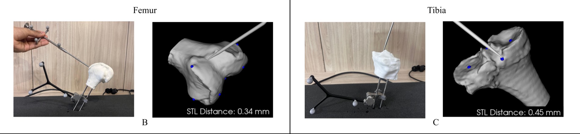
The conclusion the authors do draw: MBEDNet matches, and in places outperforms, existing state-of-the-art architectures at a lower computational cost, and stays diagnostically reliable in advanced disease — giving surgeons accurate preoperative masks regardless of severity.
@inproceedings{mbednet,
  title     = {MBEDNet: A Mamba-CNN Network with Dual Edge-Guided
               Decoders for Segmentation of TibioFemoral Bone
               and Cartilage},
  author    = {Anonymized Authors},
  note      = {Under double-blind review},
  url       = {https://anonymous.4open.science/r/MBEDNet-D6EC}
}
Author and venue fields are withheld while the submission is under double-blind review.